Credit Risk Pipeline on Databricks

End-to-end default prediction for a simulated South African lender

A bronze/silver/gold lakehouse pipeline on Databricks that cleans messy lending data, builds a leakage-free loan table and trains MLflow-tracked default models, with a portfolio risk dashboard.

NoteAt a glance

• Data: 9,564 loans across six simulated source tables (customers, applications, loans, repayments, partners, campaigns)
• Pipeline: bronze → silver → gold Delta tables on Databricks, with automated data quality checks
• Model: logistic regression, AUC 0.668 / Gini 0.336 on a time-based holdout of 1,256 loans
• Tools: Databricks, PySpark, Delta Lake, SQL, scikit-learn, MLflow, Databricks AI/BI

View the code on GitHub Open the live dashboard

All data in this project is simulated. It is built to behave like a South African consumer lender’s portfolio, including the data quality problems real source systems have.

Why I built this

Most of my work so far has been in clinical genomics and tuberculosis research. I wanted a project that showed the same skills (messy data, careful pipelines, honest modelling) applied to a business problem, and credit risk is one of the most common uses of data science in South African banking and insurance.

The lender in this project needs to answer three questions:

1. Which applicants are likely to default? A model that ranks new applicants by risk at the point of application.
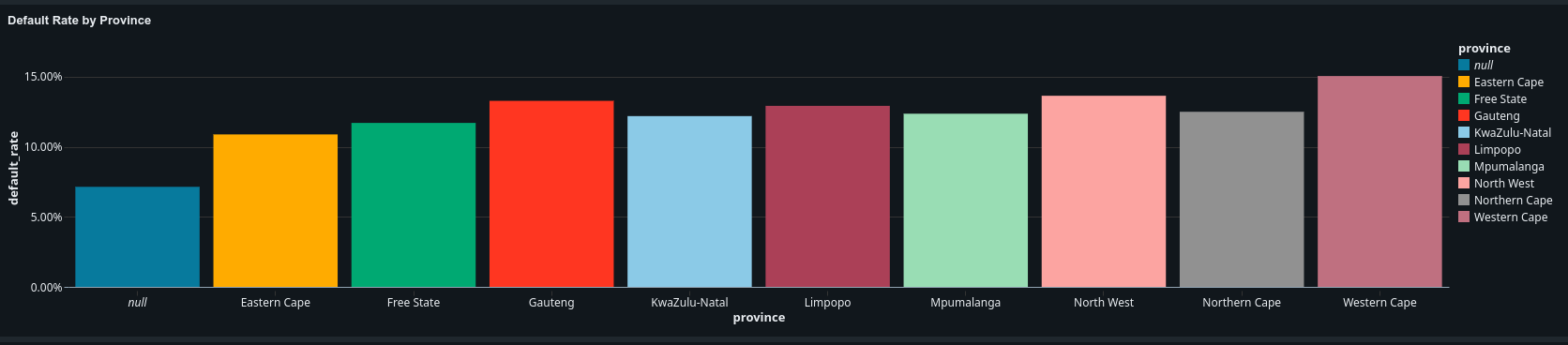
2. Where is the portfolio risk concentrated? Default rates by province, channel and time.
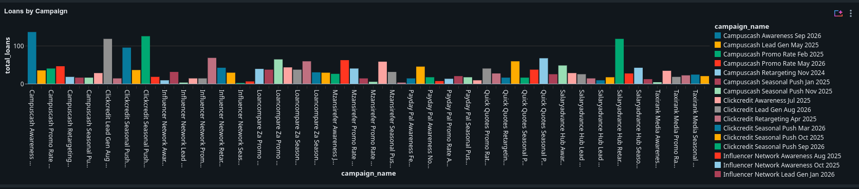
3. Which marketing campaigns are worth the money? Cost per application and cost per approved loan.

Architecture

flowchart LR
    A[Source files] --> B[Bronze<br/>raw + lineage]
    B --> C[Silver<br/>cleaned and validated]
    C --> D[Gold<br/>model-ready tables]
    D --> E[Models<br/>MLflow]
    D --> F[Dashboard and<br/>risk report]
    E --> F

Layer	What happens
Bronze	Source files loaded as-is, with lineage columns recording the source file, sheet and ingestion time
Silver	IDs standardised, money, numbers and dates parsed, categories mapped, out-of-range values nulled, duplicates removed, quality checks enforced
Gold	One row per loan with application-time features and a default label, plus campaign attribution and efficiency tables
Model	Time-based train/test split, two models compared, metrics and models logged to MLflow

One notebook, 00_run_all, runs every stage in order and prints a summary of the gold table and the latest model results.

Cleaning messy data

The source data has the kinds of problems real lending data has. Rather than fixing them ad hoc, I wrote shared functions in src/cleaning.py that every notebook uses.

Problem in the source	How the pipeline handles it
IDs written as c00042, C 0042, 42	Standardised to C00042
Money as R 7350, R7,350, 7350.00	Currency symbols, spaces and commas stripped
Dates in seven formats, some with two-digit years	Each format tried in turn; dates outside a valid range rejected
Null markers such as N/A, ND, unknown, -	Recognised by one shared pattern and treated as missing
Free-text categories (gau, Gauteng, GAUTENG)	Mapped to standard values; ambiguous ones (Nor) reported and left blank rather than guessed
Campaigns with swapped dates or negative spend	Corrected and flagged

For example, a single function handles every money format:

def parse_money(df, c):
    """'R 7350', 'R7,350', '7350.00' -> 7350.0"""
    t = F.regexp_replace(F.trim(F.col(c)), r"[Rr,\s]", "")
    return df.withColumn(
        c,
        F.when(F.col(c).rlike(NULL_TOKENS), F.lit(None).cast("double"))
         .otherwise(t.try_cast("double")),
    )

Every silver table must also pass checks before it is written: unique keys, no unparsed dates, and no orphaned records (for example, repayments for a loan that does not exist). If a check fails, the pipeline stops, so bad data never reaches the gold layer.

Building a leakage-free loan table

The gold layer is where most of the modelling decisions live. Three of them matter most.

1. Only use what was known at application time. For example, the number of previous applications counts only those made before the current one:

w = (Window.partitionBy("customer_id")
     .orderBy("application_date", "application_id")
     .rowsBetween(Window.unboundedPreceding, -1))
apps = apps.withColumn("n_prior_applications", F.count("*").over(w))

2. A clear definition of default. A loan counts as defaulted if it reaches 90+ days past due within its first 6 instalments, or within the full term for shorter loans.

3. Only label loans that have been watched long enough. A loan that has defaulted after three months is easy to label, but a loan that is three months old and still paying might default next month. Labelling it “no default” too early would make recent loans look safer than they are. So loans that have not been observed for the full window get no label:

defaulted = F.col("max_dpd") >= 90
matured = F.col("n_observed") >= window_len

g = (g.withColumn("matured", F.coalesce(matured, F.lit(False)))
      .withColumn("default_flag", F.when(F.col("matured"), defaulted.cast("int"))))

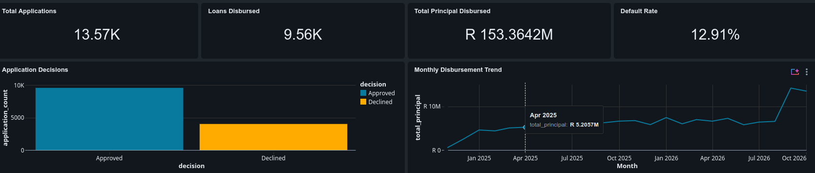
This leaves 6,276 matured loans with a 19.7% default rate for modelling, out of 9,564 in total.

Modelling

I split the data by time: the model trains on the oldest 80% of loans and is tested on the newest 20%. That is how a lender would actually use it, trained on past customers and applied to future ones. A random split would let the model learn from loans that came after the ones it is tested on.

I compared two models inside the same scikit-learn pipeline (median imputation, scaling and one-hot encoding), with every run logged to MLflow:

Model	Test AUC	Test Gini
Logistic regression	0.668	0.336
Gradient boosting	0.626	0.253

Logistic regression won. With around 5,000 training loans, gradient boosting overfits slightly, while the simpler model generalises better to new loans. Lenders also tend to prefer logistic regression, because each feature’s effect can be explained to regulators and credit committees.

Features used: loan terms (principal, term, interest rate), affordability (income, debt-to-income, loan-to-income), credit history (bureau score, no-bureau-hit flag, prior applications), applicant details (age, employment duration, employer type, province) and channel type.

TipA deliberate exclusion

Sex is in the data but not in the model. South Africa’s National Credit Act prohibits unfair discrimination in credit decisions, and a production scorecard would not use it.

Dashboard

The dashboard is built in Databricks AI/BI on the gold tables and gives a credit manager a one-page view of the portfolio.

Portfolio overview: applications, loans disbursed, principal lent, default rate, approval decisions and the monthly disbursement trend.

Loans brought in by each marketing campaign.

Default rate by province.

Borrower profile by province: bureau score, income, debt-to-income and default rate.

Loan volume by partner channel.

What I learned

• Most of the work is in the data, not the model. Cleaning six messy tables and getting the label right took far longer than training, and mattered more for the result.
• Data leakage hides in ordinary-looking choices. Using a random split, or labelling recent loans as non-defaulters, would both have produced a better-looking score that would not hold up in practice.
• Simpler can be better. The more complex model scored lower on future loans.
• Shared, tested functions pay off. Writing the cleaning and quality checks once and reusing them made the pipeline easier to debug and rerun.

Next steps

• Improve the features, compare a binned (weight-of-evidence) scorecard, and tune hyperparameters
• Check calibration, so predicted default probabilities match observed default rates
• Schedule the pipeline as a Databricks job, with monitoring for data drift and model performance